From causal inference to autoencoders and gene regulation by Caroline Uhler

From causal inference to autoencoders and gene regulation by Caroline Uhler#

Posted on 2019-11-16

Disclaimer: These notes are based on my frantic scribbling from this one talk and will most certainly contains misunderstandings even though I’ve tried my best to stay true to the original content.

Caroline Uhler gave a very interesting talk this Friday ³ ³For an almost identical talk see her talk at ICML 2019. that went from the very practically motivated problem of studying genes all the way down to characterizing overparameterization of neural network theory.

The talk was given in the backlit of the scientific opportunity which comes with having high-throughput observation and interventional single-cell gene expression ¹ ¹It is still unclear to me what exactly we observe as a gene expression. However, I imagine that the reason we model this as a causal network is because a particular gene could impact to what degree other genes are being read. So the genes do not have a causal relation directly by the expression of them does. data available. Let us unpack that a little to appreciate it: we have roughly 20,000 genes in each cell. For one of those cells we can quickly obtain 100,000 to 1 mio. observations (see Fig. 1). Not only that, we can even knock out a particular gene thanks to the CRISPR-seq method. These kinds of large-scale studies have previously not been possible – this would for instance be ethically problematic when testing medicine on human groups. So the problem of what can asymptotically be learned for different kinds of interventions has only recently become interesting practically.

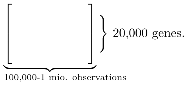
../../_images/data.png — Fig. 1 **Data matrix** The observations can be represented by data matrix where each column consistent of 20,000 values – one for each gene. Most of the entries are zero entries because of the high level of noise in the measurements.#

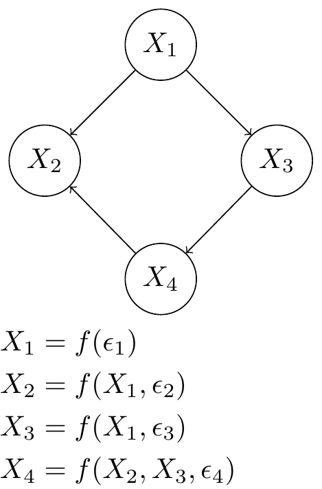
../../_images/GRN.png — Fig. 2 **A Gene Regulatory Network** of 4 genes represented by random variables in a Bayesian Network. Each random variable is a function of some noise and the other random variables dictated by network structure. The graphical model and structure equation model are equivalent.#

These gene expression observations can be viewed as a causal system – in this setting specifically referred to as a Gene Regulatory Network. Each observation column in the data matrix is a realization of a collection of random variable whose correlation structure can be captured by a directed acyclic graph (DAG) also known as a Bayesian Network. We are ultimately interested in finding the unique network which governs our data (see Fig. 3). It is well known that we would not be able to uniquely identify the network by observational data alone since correlation is a symmetric relation. So we need to interact with the system, i.e. perturb it. The question is how much we can narrow down the network structure.

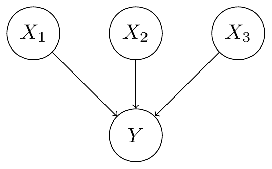
../../_images/trait_cause.png — Fig. 3 **Trait causes** Note that this problem is different from learning the causes of traits. That problem is much simpler as the network reduces to the network structure illustrated below.#

Interventional data#

It is useful to consider two types of interventions (also known as perturbations):

perfect or hard intervention in which one of the random variable is made fixed,

\[X_2 = c.\]

This corresponds to deleting on incoming edges to \(X_2\).
imperfect intervention in which the random variable is modified,

\[X_2 = \tilde{f}(X_1, \tilde{\epsilon}_2).\]

Studying the effect of these perturbations was divided into roughly three parts:

What causal structures is it even possible to distinguish between with interventional data?
How do we construct an algorithm for learning the class of graphs that can lead to the observed data?
How do we optimaly pick the intervention to narrow down the graph? (this is still an open question.)

Markov equivalent classes (identifiability)#

The so called markov equivalence classes have already been characterized for observational data. That is, the set of graphs that are indistinguishable by only using observational data (see Fig. 4 for an example). Obviously when additionally using interventional data we can still distinguish between graphs that where possible with observational data alone. But can we divide these sets further? It turns out that with interventions we can distinguish between:

the same as for observational and
adjacent to intervention nodes.

This turns out to be true even for imperfect interventions (but it comes at a computational cost). This is of high practical relevance since for cell perturbations a hard intervention would mean killing the cell. An imperfect intervention on the other hand would only kill off the cell with high probability after roughly 5 interventions. This allow us to distinguish between many more graph than if we could only perform one intervention.

../../_images/markov-eq-classes.gif — Fig. 4 The markov equivalence classes for a three node graphs when using observational data. (source)#

Learning the DAG#

It is not too difficult to show that we can reduce the learning of this Directed Acyclic Graph (DAG) into two independent sub-problems:

²Notice that the nodes in every DAG can be ordered such that all edges points in one particular direction. Intuitively learning the order reduces the space of possible DAGs to search.

First we learn an ordering of nodes ² ²Notice that the nodes in every DAG can be ordered such that all edges points in one particular direction. Intuitively learning the order reduces the space of possible DAGs to search..
Then we learn the corresponding DAG.

The second problem was already solve so this separation reduced the task to learning the right ordering.

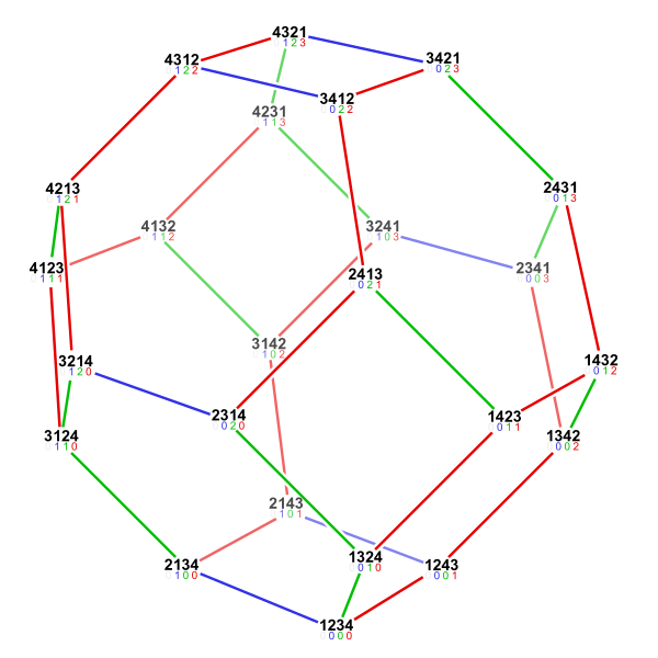
Permutohedron The space of possible orderings can be captured by a \((n-1)\)-dimensional polytope where each node is a unique permutation (see Fig. 5). An edge exists between two nodes if you can get to one from another by a adjacent transposition leading to \((n-1)\) edges for each node.

../../_images/permutohedron.png — Fig. 5 The permutohedron (source).#

It turns out that for observational data a simple greedy algorithm which traverses this polytope is sufficient for learning the ordering. Formally we need to show that our algorithm is provably consistent. That is, in the limit of infinite steps it converges to the right ordering no matter the starting point in this polytope ⁴ ⁴To obtain an efficient algorithm they further showed that a sparse polytope is sufficient..

Learning for interventions Now for interventional data the story is different:

For perfect interventions this correspond to pruning the polytope by cutting off edges to intervened targets. This is not consistant in general which is quite intuitive.
For imperfect interventions_ on the other hand we can obtain consistancy which gives us hope even if the assymptotic convergence is slow.

Where should we intervene#

The last point concerning genetics was mostly a cry for help. We have so far only considered knocking out single genes and analysed what causal structure we can infer given a fixed interventional data set. Two exciting and big open problems concerns knocking out multiple genes and how to choose the imperfect interventions.

Auto-Encoder Theory#

In the second part of her talk she left the genetics behind and instead talked about cancerous cells. Detecting cancers is an important problem where current attempt at automating the process relies on labeled data curated by practitioners. A naive approach would use this data set to at best replicate the performance of practitioners. Uhler on the other hand had the ambitious goal of detecting teh cancerous cells before it was humanly possible.

Going back in time She manages this by training and a Variational Auto-Encoder (VAE). Through that she obtains a low dimensional (probabilistic) embedding of each cell. Given a timeseries of pictures for a cell she then proceeds by learning the time-evolution in this lower dimensional space. Specifically, she learns the Optimal Transport map from one cell embedding to the next. Inverting this mapping (which is a \(m\times m\)-matrix where \(m\) is the dimensionality of the latent space). Not only did this provide a way to step back in time but she additionally use it to exterpolate ⁵ ⁵It was a little unclear to what extend they manage to distinguish cancerous cells before experts. Especially since it is not obvious how to evaluate your performance – after all no baseline exists that you can compare yourself against. ⁶ ⁶The details of the method can be found on bioRxiv. It seems to be an early draft with the mathematical details showing quite a bit into it in the supplementary material..

Auto-encoders What I found even more fascinating with this use of Auto-encoders (AE) here was that it motivated a theoretical study of AE which lead to very general results. In particular, her group showed that an overparameterized AE ⁷ ⁷Note that there is a slight discrepancy here: the study on overparameterization is done in the context of Auto-Encoders not Variational Auto-Encoders as used in the cancer application. Even though the difference might seem subtle at first sight my understanding is that they are treated as two very different mathematical objects. network generalizes well because it memorizes the training data and interpolate between the points.

A contracting map In the process they even devised a procedure for extracting the training examples. This is done by simply re-applying the network repeatedly to the previous output of the network. Practically this procedure is possible since the input and output space is the same for an Auto-Encoder. In the terminology of dynamic system theory the AE is a contracting map.

This has profound practical consequences and is both a blessing and a curse. On the one hand, this is exactly what makes Auto-Encoder work when overparameterized as is standard practise. On the flipside, this raises real privacy concerns: Medical application using AE are bound to leak confidential patient data to the people with access to the model.

A linear algebra perspective They approached the understanding of overparameterized AE very methodically. First they verified that it did not simply learn an identity map. In particular, they fed a trained network completely random noise and observed that the network produced images close to the training images. This was the first proof that something curious was going on. That let them to theoretically study the problem. They first showed that when restricted to linear mappings the network learns the lowest dimensional projection and that the output will lie in the span of training data. They then managed to obtain analogies results to this for non-linear mapping ⁸ ⁸From what I understand they actually manage to understand the overparameterized setting for Autoencoder fully. I would like to understand the details however, since for neural networks as function approximators the interest is in the degree of overparameterization. I don’t know whether what they have obtain is in some way tight.. This is yet another example of how useful it is to first reason about a problem under the simplifying assumption of linearity.

Practical advice These theoretical results explains the necessity for overparameterization of autoencoders – in some way the network becomes more regularized. For CNN they obtained results that this corresponds to adding depth since it can be shown that width does not give you so much more expressive power.

Final Remarks#

It was incredible seeing this biological application driving results in two distinct theoretical fields: causal inference and neural network theory. The AE result is one of those results that in hindsight seems so obvious.