The I/O Model#
Posted on 2018-05-22
Usually when we analyse the running time of algorithm we consider the number of CPU cycles it requires. However, this assumes that the reading and writing to memory is as cheap as some computation performed by the CPU. In reality accessing memory is cheap, but if the problem size (or the generated data) is so massive that it cannot fit into memory, we will have to write to external storage. The properties of this external storage is that even though we have a lot of it (almost unbounded), it is orders of magnitudes slower than the RAM. So if we are counting both external storage accesses and CPU cycles, the CPU cycles contributes almost nothing to the total. Thus for very big problem it makes sense to analyse them in terms of the number of external storage accesses it does and completely disregard CPU cycles. This is what is called the I/O model and we will see how this different way of counting influences our algorithmic design.
Computations Models#
To define more formally these different ways of analyzing an algorithm, let us consider first how a simplified computer is structured. The general structure is shown in Fig. 6 having two caches close to the CPU followed by a Random Access Memory (RAM) and furthest away the disk storage. RAM is much faster than disk storage but expensive which is why it is limited in size. Disk storage, on the other hand, is slow but cheap which is why we have a lot. As indicated by the distance from the CPU the disk is much slower to access.

Fig. 6 Structure of a physical computer. Longer distances means longer access time while width denotes space. The layers \(L1\) and \(L2\) are examples of caching layers that can fit in less data than the RAM but provides faster access.#
There are two simplifying models we will consider to approximate how things are in reality. The first model we considered, called the RAM model, assumes that everything can fit in memory (formally that we have unbounded memory).
Definition 4 (RAM model)
This hypothetical computer makes two assumptions:
Each memory access and simple operation (e.g. arithmetic, boolean operators, function calls) takes exactly 1 time step.
The memory is unbounded.
The cost is number of timesteps.
What the I/O model instead counts is only the read/write operations to disk.
Definition 5 (I/O model)
The model assumes:
Problem size is \(N\).
Limited memory of size \(M\).
Infinite disk space.
And I/O operation read/write a consecutive block of \(B\) between memory and disk.
Computation can only be done on cells in memory.
The cost is only the number of I/O’s operations (as a function of \(N\), \(M\) and \(B\)) so computations are free.
Even though the I/O model is still an oversimplification of the actual architecture it has shown to predict the asymptotic running time accurately in many cases.
We will consider how to obtain efficient sorting in the I/O model.
Sorting#
One merge algorithm that can be adjusted to be efficient for the I/O model is the mergesort algorithm, specifically a \((M/B)\)-way mergesorting [Aggarwal and Vitter, 1988].
Merge#
The objective is to merge a number of sorted arrays together. Say we want to keep one block for each array in memory at every given time then we can only merge \(M/B\) sorted arrays if using a multi-array merge.
The \((M/B)\)-way merge proceed as follows. We merge the usual way by maintaining a pointer for each array starting at the first index. We then take the minimum value of the pointers and increment the pointer at the minimum value. The different is that if the pointer overflows the currently loaded block for the given array the next block in the array is loaded instead. Additionally, when the output in memory reaches a size of \(B\) it is written to disk and removed from memory.
Correctness The argument for correctness is similar to normal \(k\)-way merge but we also have to consider whether enough memory is available. Fortunately, we can keep all \(M/B\) array of size \(B\) in memory since they take up \(O(M/B)O(B)=O(M)\) in total.
I/O Complexity Here we use that we have divided the input arrays and output array into chunks of size \(B\). The arrays are divided into \(N/B\) blocks and the output is written using \(N/B\) blocks. So \(O(N/B)\) I/O operations are spent.
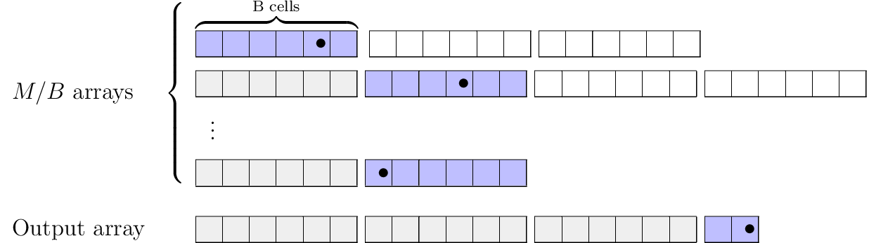
Fig. 7 \(M/B\)-way merge.
 indicates blocks that have already been in memory.
 indicates blocks that are currently in memory.
 denotes the current pointer for the array.#
Sort#
The merging step requires already sorted arrays. Observe that we can sort \(M\) cells at a time efficiently since computations are free when the cells fit in memory.
So to turn an unsorted array of length \(N\) into \(N/M\) sorted arrays (each of length \(M\)) first load in \(M\) cells using \(M/B\) blocks and sort them using some sorting algorithm. Do this for all \(N/M\) sub arrays.
I/O Complexity Each sub array takes \(M/B\) I/O reads and writes, and there are \(N/M\) block so number of I/O operations is \(O((M/B)(N/M)) = O(N/B)\).
Mergesort#
Now, the idea is that we can combine the sorting and merging step to get an efficient mergesort in the I/O model.
Apply Sort to get \(N/M\) sorted arrays of length \(M\). Now, iteratively merge bundles of \(M/B\) arrays so that the number of arrays at each level is reduced by \(M/B\).
Complexity To figure out the complexity for the entire computational tree (illustrated in Fig. 8) we analyse how much each layer uses and how many layers we have.
How many I/O operations are used on each level? We count the level index from above. There are \((M/B)^i\) arrays in total at level \(i\) each having size \(N/(M/B)^i\) thus taking \(\frac{N/(M/B)^i}{B}\) operations to sort using Merge. In total \((M/B)^i\frac{N/(M/B)^i}{B}=N/B\).
How many levels are needed? The number of arrays at level \(i\) is \((M/B)^i\). When this is equal to \(N/M\) we can apply Sort. Solving for \(i\) yields:
So we spend \(N/B\) for each \(\log_{M/B}{N/M}\) levels and apply Sort once on the final level taking \(O(N/B)\). Number of I/O is thus
which is actually a closer bound than what the article suggests.
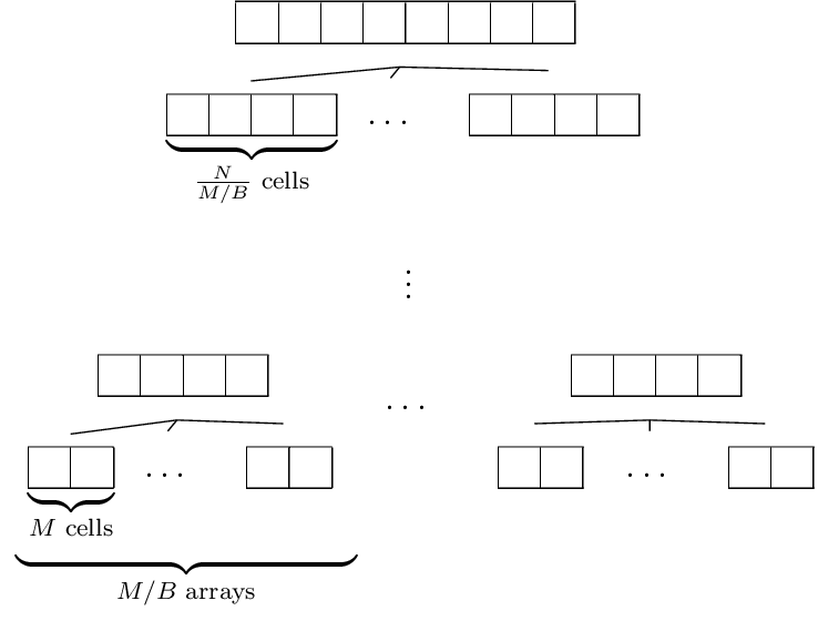
Fig. 8 Mergesort that sorts arrays in the bottom layer using Sort and then merging bundles of \(M/B\) sorted arrays recursively until only one sorted array of length \(N\) is left.#
Conclusion#
We have introduced the I/O model and shown an efficient mergesort algorithm when \(N \gg M\). It has very similar running time as the standard mergesort with \(O(n \log n)\) but it differs by depending on \(B\) and \(M\). Specifically it makes \(O(N/B \log_{M/B}(N/M))\) I/O operations.
Next we will explore what we can do if we do not know \(M\) and \(B\).
- AV88
Alok Aggarwal and S. Vitter, Jeffrey. The input/output complexity of sorting and related problems. Commun. ACM, 31(9):1116–1127, September 1988. URL: http://doi.acm.org/10.1145/48529.48535, doi:10.1145/48529.48535.
Cite this post#
@misc{pethick2018iomodel,
  author = {Thomas Pethick},
  title = {The I/O Model},
  year = {2018},
  month = {05},
  day = {22},
  url = {https://pethick.dk/posts/2018-05-22-io-model/},
  note = {Blog post}
}